Chapter 5.2 Fault-tolerant Quantum Transformer

This content of this section corresponds to the Chapter 5.2 of our paper. Please refer to the original paper for more details.

In this section, we move on to show an end-to-end transformer architecture implementable on a quantum device, which includes all the key building blocks introduced in Chapter 5.1, and a discussion of the potential runtime speedups of this quantum model. In particular, here we focus on the inference process in which a classical Transformer has already been trained and is queried to predict the single next token.

Recall that in Chapter 5.1, we suppose that the three parameterized matrices in the self-attention mechanism have the same size, i.e., $W_q, W_k, W_v \in \mathbb{R}^{d \times d}$. Besides, the input sequence $S$ and the matrix returned by the attention block $G^{\text{soft}}$ has the size $\ell \times d$. Here, we further suppose the length of the sentence and the dimension of hidden features exponentially scale with $2$, i.e., $\ell=2^N$ and $\log d\in \mathbb{N^+}$. This setting aligns with the scaling of quantum computing, making it easier to understand. For other cases, padding techniques can be applied to expand the matrix and vector dimensions to conform to this requirement.

Since the runtime speedups depend heavily on the capabilities of the available input oracles, it is essential to specify the input oracles used in the quantum Transformer before detailing the algorithms. For the classical Transformers, the memory access to the inputs such as the sentence and the query, key, and value matrices is assumed. In the quantum version, we assume the access of several matrices via block encodings introduced in Chapter 2.4.

Assumption 5.2.1. Following the explicit form of the single-head and single-layer Transformer, there are five parameterized weight matrices, i.e., $W_q$, $W_k$, $W_v \in \mathbb{R}^{d\times d}$ in the attention block, as well as $M_1\in \mathbb R^{d’ \times d}$ and $M_2 \in \mathbb R^{d \times d’}$ in FFN. Note that here, $M_1$ and $M_2$ is actually the transpose of parameterized matrices in the classical transformer. Quantum Transformer assumes access to these five parameterized weight matrices, as well as the input sequence $S\in \mathbb{R}^{\ell \times d}$ via block encoding.

Mathematically, given any $A\in {W_q, W_k, W_v, M_1, M_2, S}$ corresponding to an $N$-qubit operator, $\alpha, \varepsilon\geq 0$ and $a\in \mathbb{N}$, there exists a $(a+ N)$-qubit unitary $U_A$ referring to the $(\alpha,a,\varepsilon)$-block-encoding of $A$ with

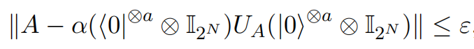
where $|\cdot|$ represents the spectral norm.

Under this assumption, we know that the quantum Transformer can access $U_S$, $U_{W_q}$, $U_{W_k}$, and $U_{W_v}$ corresponding to the $(\alpha_s,a_s)$-encoding of $S$ and $(\alpha_w,a_w)$-encodings of $W_q,W_k$ and $W_v$, respectively. Moreover, the quantum Transformer can access $(\alpha_{m},a_{m})$-encodings $U_{M_1}$ and $U_{M_2}$ corresponding two weight matrices $M_1\in \mathbb R^{d’ \times d}$ and $M_2 \in \mathbb R^{d \times d’}$ in FFN.

For simplicity and clarity, in the following, we consider the perfect block encoding of input matrices without errors, i.e., $\varepsilon=0$. As such, we will not explicitly write the error term of the block encoding, and use $(\alpha,a)$ instead of $(\alpha, a,0)$. The output of quantum transformer is a quantum state corresponding to the probability distribution of the next token. The complete single-layer structure is described in Figure 5.2.

Under the above assumptions about access to the read-in protocols, the following theorem indicates how to implement a single-layer transformer architecture on the quantum computer.

Theorem 5.1. For a single-layer and single-head Transformer depicted in Figure 5.2, suppose its embedding dimension is $d$ and its input sequence $S$ has the length $\ell=2^N$. Under Assumption 5.2.1 about the input oracles, for the index $j\in [\ell]$, one can construct an $\epsilon$-accurate quantum circuit for the quantum state proportional to $$\begin{aligned} \sum_{k=1}^d \mathrm{Transformer}(S,j)_k \ket{k}, \end{aligned}$$ by using ${\mathcal{\tilde{O}}}(d N^2 \alpha_s\alpha_w \log^2(1/\epsilon))$ times of the input block encodings.

We show this theorem by explicitly designing the quantum circuit for each computation block of the transformer architecture in a coherent way, i.e., without intermediate measurement. The quantum circuit can be used for subsequent layers. In addition, a subsequent transformation of the amplitude-encoded state and measuring in the computational basis outputs the index of the next predicted token according to the probabilities modeled by the transformer architecture.

Roadmap. In our paper, we detail the implementation of quantum Transformers, proceeding from the bottom to the top as illustrated in Figure 5.2. Specifically, we first demonstrate how to quantize the attention block. Next, we present the quantization of residual connections and layer normalization operations. Last, we exhibit the quantization of the fully connected neural network to complete the computation $\mathrm{LN}(\mathrm{FFN}(\mathrm{LN}(\mathrm{Attention}(S,j))))$. Please refer to the original paper for details.