Chapter 4.4 Theoretical Foundations of QNNs

This content of this section corresponds to the Chapter 4.4 of our paper. Please refer to the original paper for more details.

As a machine learning (ML) model, the primary goal of quantum neural networks (QNNs) is to make accurate predictions on unseen data. Achieving this goal depends on three key factors: expressivity, generalization ability, and trainability. A thorough understanding of these factors is crucial for evaluating the potential advantages and limitations of QNNs compared to classical ML models. Instead of providing an exhaustive review of all theoretical results, this section focuses on near-term QNNs, emphasizing key conceptual insights into their capabilities and limitations.

Expressivity and generalization of quantum neural networks

The expressivity and generalization are deeply interconnected within the framework of statistical learning theory for understanding the prediction ability of any learning model. To better understand these two terms in the context of quantum neural networks, we first review the framework of empirical risk minimization (ERM), which is a popular framework for analyzing these abilities in statistical learning theory.

Consider the training dataset $\mathcal{D} = \{(\bm{x}^{(i)},\bm{y}^{(i)})\} \in \mathcal{X} \times \mathcal{Y}$ sampled independentaly from an unknown distribution $\mathcal{P}$, a learning algorithm $\mathcal{A}$ aims to use the dataset $\mathcal{D}$ to infer a hypotheis $h_{\bm{\theta}^*}: \mathcal{X}\to \mathcal{Y}$ from the hypothesis space $\mathcal{H}$ that could accurately predict all labels of $\bm{x}\in \mathcal{X}$ following the distribution $\mathcal{P}$. Under the framework of ERM, this is equivalent to identifying an optimal hypothesis in $\mathcal{H}$ minimizing the expected risk

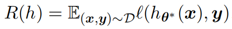
where $\ell(\cdot,\cdot)$ refers to the per-sample loss predefined by the learner. Unfortunately, the inaccessible distribution $\mathcal{P}$ forbids us to assess the expected risk directly. In practice, $\mathcal{A}$ alternatively learns an empirical hypothesis $h_{\hat{\bm{\theta}}} \in \mathcal{H}$, as the global minimizer of the (regularized) loss function $$\mathcal{L}(\bm{\theta}, \mathcal{D}) = \frac{1}{|\mathcal{D}|} \sum_{i=1}^{|\mathcal{D}|} \ell (h_{\bm{\theta}}(\bm{x}^{(i)}), \bm{y}^{(i)}) + \mathcal{R}(\bm{\theta}),$$ where $\mathcal{R}(\bm{\theta})$ refers to an optional regularizer, as will be detailed in the following. Moreover, the first term on the right-hand side refers to the empirical risk $$R_{\text{ERM}}(h_{\hat{\bm{\theta}}})= \frac{1}{|\mathcal{D}|} \sum_{i=1}^{|\mathcal{D}|} \ell (h_{\hat{\bm{\theta}}}(\bm{x}^{(i)}), \bm{y}^{(i)}),$$ which is also known as the training error. To address the intractability of $R(h_{\hat{\bm{\theta}}})$, one can decompose it into two measurable terms, $$ R(h_{\hat{\bm{\theta}}}) = R_{\text{ERM}}(h_{\hat{\bm{\theta}}}) + R_{\text{Gene}}(h_{\hat{\bm{\theta}}}),$$ where $R_{\text{Gene}}(h_{\hat{\bm{\theta}}}) = R(h_{\hat{\bm{\theta}}}) - R_{\text{ERM}}(h_{\hat{\bm{\theta}}})$ refers to the generalization error. In this regard, achieving a small prediction error requires the learning model to achieve both a small training error and a small generalization error.

Expressivity of QNNs

In this chapter, we analyze the generalization error of QNNs through a specific measure of model complexity: the covering number. By leveraging this measure, we aim to understand better and characterize the generalization performance of QNNs.

To elucidate the specific definition of the covering number, we first review the general structures of QNNs. Define $\rho\in \mathbb{C}^{2^N \times 2^N}$ as the $N$-qubit input quantum states, $O\in \mathbb{C}^{2^N \times 2^N}$ as the quantum observable, $U(\bm{\theta})=\prod_{l=1}^{N_g} u_{l}(\bm{\theta}) \in \mathcal{U}(2^N)$ as the applied ansatz, where $\bm{\theta}\in \Theta$ are the trainable parameters living in the parameter space $\Theta$, $u_{l}(\bm{\theta}) \in \mathcal{U}(2^k)$ refers to the $l$-th quantum gate operated with at most $k$-qubits with $k\le N$, and $\mathcal{U}(2^N)$ stands for the unitary group in dimension $2^N$. In general, $U(\bm{\theta})$ is formed by $N_{gt}$ trainable gates and $N_g-N_{gt}$ fixed gates, e.g., $\Theta \subset [0, 2\pi)^{N_{gt}}$. Under the above definitions, the explicit form of the output of the quantum circuit under the noiseless scenarios is $$h(\bm{\theta},O,\rho):= \text{Tr}\left( U(\bm{\theta})^{\dagger} O U(\bm{\theta}) \rho \right).$$ Given the training data set ${(\rho^{(i)}, \bm{y}^{(i)})}$ and loss function $\mathcal{L}(\cdot)$, the quantum neural network is optimized to find a good approximation $h^*(\bm{\theta},O,\rho)= \arg \min_{h(\bm{\theta},O,\rho) \in \mathcal{H}}$ that can well approximate the target concept, where $\mathcal{H}$ refers to the hypothesis space of QNNs with

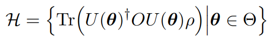
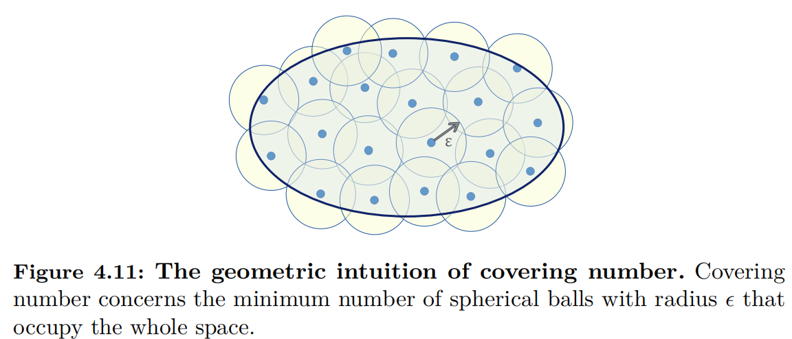
When $\mathcal{H}$ has a modest size and covers the target concepts, the estimated hypothesis could well approximate the target concept. By contrast, when the complexity of $\mathcal{H}$ is too low, there exists a large gap between the estimated hypothesis and the target concept. An effective measure to evaluate the complexity of $\mathcal{H}$ is covering number shown in Figure 4.11, an advanced tool broadly used in statistical learning theory, to bound the complexity of $\mathcal{H}$ and measure the expressivity of QNNs.

Generalization error of QNNs

As the relation between generalization error and covering number is well-established in statistical learning theory, we can directly obtain the generalization error bound with the above bounds of covering number following the same conventions.

Theorem 4.6. Assume that the loss function $\ell$ is $L_1$-Lipschitz and upper bounded by a constant $C$, the QNN-based learning algorithm outputs a hypothesis $h_{\hat{\bm{\theta}}}$ from the training dataset $\mathcal{S}$ of size $n$. Following the notations of risk $R_{\text{Gene}}(h_{\hat{\bm{\theta}}})=R(h_{\hat{\bm{\theta}}})-R_{\text{ERM}}(h_{\hat{\bm{\theta}}})$, for $0<\epsilon<1/10$, with probability at least $1-\delta$ with $\delta \in (0,1)$, we have

$$R_{\text{Gene}}(h_{\hat{\bm{\theta}}}) \le \mathcal{O}\left(\frac{8L+c+24L \sqrt{N_{gt}}\cdot 2^k}{\sqrt{n}} \right).$$

The assumption used in this analysis is quite mild, as the loss functions in QNNs are generally Lipschitz continuous and can be bounded above by a constant $C$. This property has been broadly employed to understand the capability of QNNs. The results obtained have three key implications. First, the generalization bound exhibits an exponential dependence on the term $k$ and a sublinear dependence on the number of trainable quantum gates $N_{gt}$. This observation reflects the quantum version of Occam’s razor [@haussler1987occam], where the parsimony of the output hypothesis implies greater predictive power. Second, increasing the number of training examples $n$ improves the generalization bound. This suggests that incorporating more training data is essential for optimizing complex quantum circuits. Lastly, the sublinear dependence on $N_{gt}$ may limit our ability to accurately assess the generalization performance of overparameterized QNNs [@larocca2023theory]. Together, these implications provide valuable insights for designing more powerful QNNs.

Trainability of quantum neural networks

The parameters in QNNs are trained using gradient-based optimizers such as gradient descent. Therefore, the magnitude of the gradient plays a crucial role in the trainability of QNNs. Specifically, large gradients are desirable, as they allow the loss function to decrease rapidly and consistently. However, this favorable property does not hold across a wide range of problem settings. In contrast, training QNNs usually encounters the barren plateau (BP) problem [@mcclean2018barren], , the variance of the gradient, on average, decreases exponentially as the number of qubits increases. In this section, we first introduce an example demonstrating how quantum circuits that form unitary $2$-designs [@dankert2009exact] lead to BP, and then discuss several techniques to avoid or mitigate its impact.