Chapter 4.3 Near-term quantum neural networks

This content of this section corresponds to the Chapter 4.3 of our paper. Please refer to the original paper for more details.

Following recent experimental breakthroughs in superconducting quantum hardware architectures [@arute2019quantum; @acharya2024quantum; @abughanem2024ibm; @gao2024establishing], researchers have devoted considerable effort to developing and implementing quantum machine learning algorithms optimized for current and near-term quantum devices [@wang2024comprehensive]. Compared to fault-tolerant quantum computers, these devices face two primary limitations: quantum noise and circuit connectivity constraints. Regarding quantum noise, state-of-the-art devices have single-qubit gate error rates of $10^{-4} \sim 10^{-3}$ and two-qubit gate error rates of approximately $10^{-3} \sim 10^{-2}$ [@abughanem2024ibm; @gao2024establishing]. The coherence time is around $10^2 \mu s$ [@acharya2024quantum; @abughanem2024ibm; @gao2024establishing], primarily limited by decoherence in noisy quantum channels. Regarding circuit connectivity, most superconducting quantum processors employ architectures that exhibit two-dimensional connectivity patterns and their variants [@acharya2024quantum; @abughanem2024ibm; @gao2024establishing]. Gate operations between non-adjacent qubits must be executed through intermediate relay operations, leading to additional error accumulation. To address these inherent limitations, the near-term quantum neural network (QNN) framework has been proposed. Specifically, near-term QNNs are designed to perform meaningful computations using quantum circuits of limited depth.

General framework

In this section, we introduce the architecture of a basic near-term QNN. As illustrated in Figure 4.4, a basic QNN consists of three components: the input, the model circuit, and the measurement.

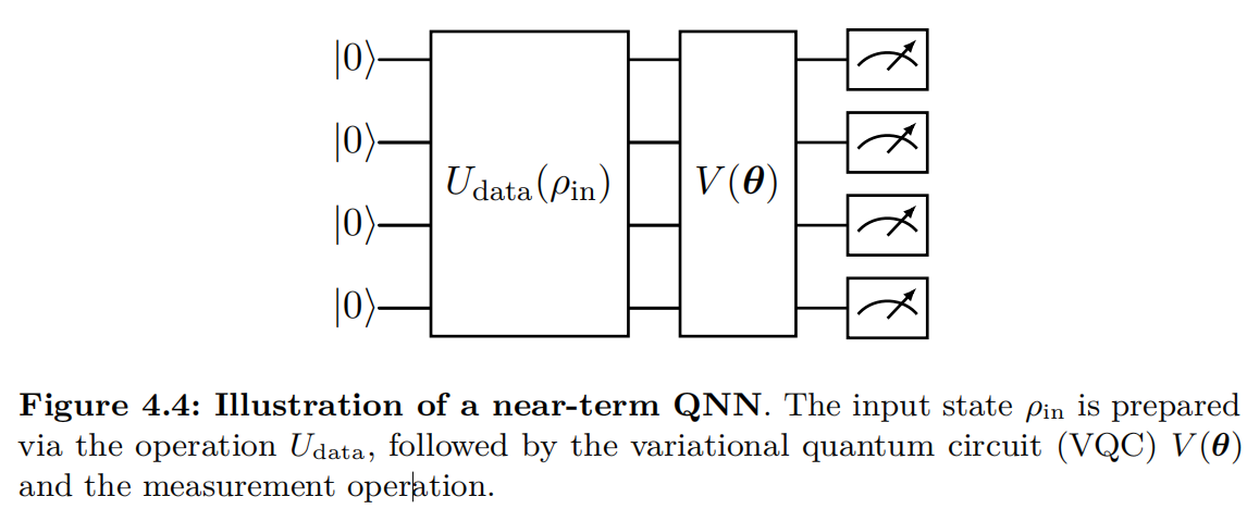
Input. The near-term QNN uses quantum states as input data. QNNs can process both classical and quantum data. Specifically, the input states $\rho_{ in}$ may be introduced from physical processes such as quantum Hamiltonian evolutions or be constructed to encode classical vectors using encoding protocols introduced in Chapter 2.3, such as angle encoding and amplitude encoding.

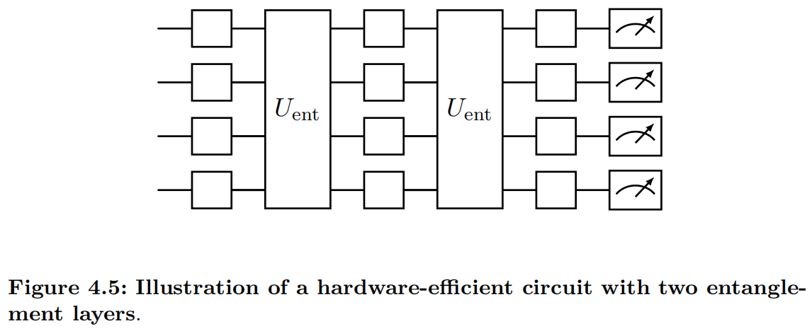
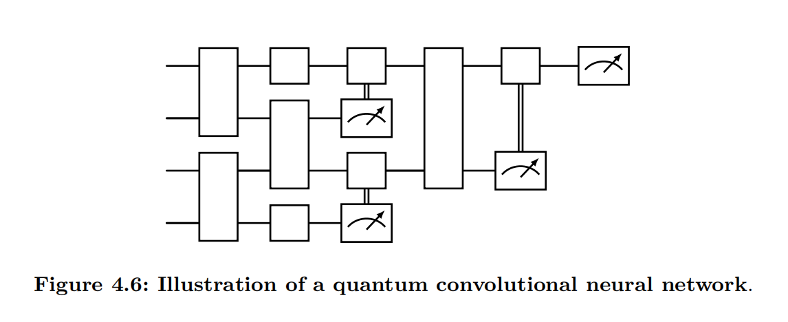
Model circuit. QNNs employ variational quantum circuits (VQCs) to extract and learn features from input data. A typical VQC, denoted as $V(\bm{\theta})$, adopts a layered architecture that consists of both parameterized and fixed quantum gates, with the former being trainable. For problem-agnostic implementations, an effective parameterization strategy is to use the parameters $\bm{\theta}$ as the phases of single-qubit rotation gates RX, RY, RZ, while quantum entanglement is introduced through fixed two-qubit gates, such as $CX$ and $CZ$. Standard circuit architectures include the hardware-efficient circuit (HEC) [@kandala2017hardware], shown in Figure 4.5, and the quantum convolutional neural network (QCNN) [@cong2019quantum], shown in Figure 4.6. For problem-specific applications, such as finding the ground states of molecular Hamiltonians, specialized circuits like the unitary coupled cluster ansatz [@peruzzo2014variational] are employed.

Measurement. After implementing the model circuit, the quantum state is measured using specific observables, denoted as $O$, to extract classical information. The choice of observables depends on the experimental objectives. In the case of a variational quantum eigensolver, where the goal is to find the ground state and energy of a given Hamiltonian, the observable is chosen to be the target Hamiltonian itself. In quantum machine learning applications involving classical data, the measurement outcomes are used to approximate label information, which typically lacks direct physical significance. As a result, the observable $O$ can, in principle, be any Hermitian operator. The measurement outcome of the near-term QNN can be expressed as a function of $\bm{\theta}$,

$$\begin{aligned} f(\bm{\theta};\rho_{ in},V,O) ={}& \text{Tr} \left[ O V(\bm{\theta}) \rho_{ in} V(\bm{\theta})^\dag \right] . \end{aligned}$$

Training of QNNs. As a QML framework, near-term quantum neural networks (QNNs) learn by optimizing parameters $\bm{\theta}$ using gradient-based methods. Therefore, the efficient computation of gradients is crucial to this approach. In particular, it is desirable to compute these gradients via quantum circuit operations. For certain cases involving parameterized gates with unitary Hamiltonians, this computation can be elegantly performed using the parameter-shift rule.

Discriminative learning with near-term QNNs

In this section, we present an example in which a near-term QNN is employed for discriminative learning. Specifically, we focus on binary classification, where the label $y^{(i)} = \pm 1$ corresponds to the input state $\rho^{(i)}$. In the case of classical data, the state $\rho^{(i)}=\ket{\psi(\bm{x}^{(i)})}\bra{\psi(\bm{x}^{(i)})}$ can be generated from the classical vector $\bm{x}^{(i)}$ using a read-in approach $$|\psi(\bm{x}^{(i)})> = U_\phi (\bm{x}^{(i)}) \ket{0} ,$$ where a simple feature map $U_\phi (\bm{x}^{(i)})$ can be constructed via angle encoding.

Denote by $O$ and $V(\bm{\theta})$ the quantum observable and the VQC, respectively. The prediction function of the near-term QNN is given by $$\hat{y}^{(i)}(\bm{\theta}) = \text{Tr} [ O V(\bm{\theta}) \rho^{(i)} V(\bm{\theta})^\dag ] .$$

In the binary classification task, the QNN learns by training the parameter $\bm{\theta}$ to minimize the distance between the label $y^{(i)}$ and the prediction $\hat{y}^{(i)}(\bm{\theta})$. Specifically, the mean square error (MSE) is used as the loss function: $$ \bm{\theta}^* = { argmin} \mathcal{L}(\bm{\theta}) , \ \text{where } \mathcal{L}(\bm{\theta}) = \sum_{i=1}^{|\mathcal{D}|} \ell (\bm{\theta}, \bm{x}^{(i)}, y^{(i)}) = \frac{1}{2} \sum_{i=1}^{|\mathcal{D}|} \left( \hat{y}^{(i)} (\bm{\theta}) - y^{(i)} \right)^2 .$$ The gradient of the loss can be calculated via the chain rule $$\nabla_{\bm{\theta}} \mathcal{L}(\bm{\theta}) = \sum_{i=1}^{|\mathcal{D}|} \left( \hat{y}^{(i)} (\bm{\theta}) - y^{(i)} \right) \nabla_{\bm{\theta}} \hat{y}^{(i)} (\bm{\theta}) ,$$ where the gradient of the prediction $\hat{y}^{(i)}$ can be obtained by using the parameter-shift rule. Consequently, a variety of gradient-based optimization algorithms, such as stochastic gradient descent, Adagrad, and Adam, can be employed to train near-term QNNs.

The QNN binary classification framework can be naturally extended to multi-label classification using the one-vs-all strategy. Specifically, we train $k$ QNN binary classifiers for $k$ classes, with each classifier distinguishing a specific class from the others.

The QNN classification framework presented in this section can be extended to quantum regression learning by incorporating continuous labels.

Generative learning with near-term QNNs

In this section, we introduce a quantum generative model based on near-term QNNs, namely the quantum generative adversarial network (QGAN) [@lloyd2018quantum]. Similar to its classical counterparts, QGAN learns to generate samples by employing a discriminator and a generator, which are engaged in a two-player minimax game. Specifically, both the discriminator $D$ and the generator $G$ can be implemented using near-term QNNs. By leveraging the expressive power of QNNs, QGAN has the potential to exhibit quantum advantages in certain tasks[@bravyi2018quantum; @zhu2022generative].

To illustrate the training and sampling processes of QGAN, we present two examples based on the quantum patch and batch GANs proposed by @huang2021experimental. Let $N$ denote the number of qubits and $M$ the number of training samples. The patch and batch strategies are designed for the cases where $N < \lceil \log M \rceil$ and $N > \lceil \log M \rceil$, respectively. Specifically, the patch strategy enables the generation of high-dimensional images with limited quantum resources, while the batch strategy facilitates parallel training when sufficient quantum resources are available.

Quantum patch GAN

We begin by introducing the quantum patch GAN, which consists of a quantum generator, as illustrated in Figure 4.7, a classical discriminator, and a classical optimizer. Both the learning and sampling processes of an image are performed in patches, involving $T$ sub-generators. For the $t$-th sub-generator, the model takes a latent state $\bm{z}$ as input and generates a sample $G_t(\bm{z})$. Specifically, the latent state is prepared from the initial state $\ket{0}^{\otimes N}$ using a single-qubit rotation layer, where the parameters are sampled from the uniform distribution over $[0,2\pi)$. The latent state is then processed through an $N$-qubit hardware-efficient circuit $U_{G_t} (\bm{\theta})$, which leads to the state $$\ket{\psi_t (\bm{z})} = U_{G_t} (\bm{\theta}) \ket{\bm{z}} .$$

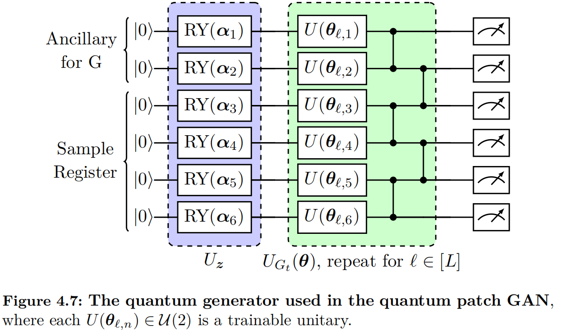
To perform non-linear operations, partial measurements are conducted, and a subsystem $\mathcal{A}$ (ancillary qubits) is traced out from the state $|\psi_t>$. The resulting mixed state is

$$\rho_t(\bm{z}) = \frac{\text{Tr}_{\mathcal{A}} \left[ \Pi \otimes \mathbb{I} |\psi_t (\bm{z}) > < \psi_t (\bm{z}) | \right] }{\text{Tr} \left[ \Pi \otimes \mathbb{I} |\psi_t (\bm{z}) > < \psi_t (\bm{z}) | \right]} ,$$

where $\Pi$ is the projective operator acting on the subsystem $\mathcal{A}$. Subsequently, the mixed state $\rho_t(\bm{z})$ is measured in the computational basis to obtain the sample $G_t(\bm{z})$. Specifically, let $P(J=j):=\text{Tr}[|j><j|\rho_t(\bm{z})]$, where the probabilities of the outcomes can be estimated by the measurement. The sample $G_t(\bm{z})$ is then defined as $$\begin{aligned} G_t(\bm{z}) ={}& [ P(J=0), \cdots, P(J=j), \cdots, P(J=2^{N-N_{\mathcal{A}}}-1) ], \end{aligned}$$ where $N_{\mathcal{A}}$ is the number of qubits in $\mathcal{A}$. Finally, the complete image is reconstructed by aggregating these samples from all sub-generators as follows: $$G(\bm{z}) = [G_1(\bm{z}), \cdots, G_T (\bm{z})] .$$

In principle, the discriminator $D$ in a quantum patch GAN can be any classical neural network that takes the training data $\bm{x}$ or the generated sample $G(\bm{z})$ as input, with the output $$D(\bm{x}), \ D(G(\bm{z})) \in [0,1] .$$ Let $\bm{\gamma}$ and $\bm{\theta}$ denote the parameters of the discriminator $D$ and the generator $G$, respectively. The optimization problem for the quantum patch GAN can be formulated as:

Similar to quantum discriminative learning, the quantum patch GAN can be trained using gradient-based optimization algorithms.

Quantum batch GAN

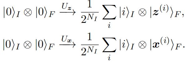
As illustrated in Figure 4.8, the quantum batch GAN differs from the quantum patch GAN by employing a quantum discriminator. In a quantum batch GAN, all qubits are divided into two registers: the index register, consisting of $N_I$ qubits, and the feature register, consisting of $N_F$ qubits. The qubits in the feature register are further partitioned into three parts: $N_D$ qubits for generating quantum samples, $N_{A_G}$ qubits for implementing non-linear operations in the generator $G_{\bm{\theta}}$, and $N_{A_D}$ qubits for implementing non-linear operations in the discriminator $D_{\bm{\gamma}}$. For a batch with size $|B_k|=2^{N_I}$, two oracles are used to encode the information of latent vectors and training samples:

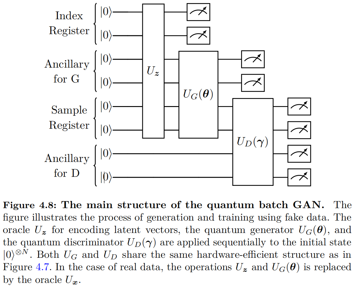
For data with $M$ features, state preparation for amplitude encoding in $U_{\bm{x}}$ requires $\tilde{\mathcal{O}}(2^{N_I}M)$ multi-controlled quantum gates, which is infeasible for current NISQ devices. This challenge can be addressed by employing pre-trained shallow circuit approximations of the given oracle [@benedetti2019generative].

After the encoding stage, a PQC $U_G(\bm{\theta})$ and the corresponding partial measurement are employed as the quantum generator. Thus, the generated state corresponding to $|B_k|$ fake samples is obtained as follows:

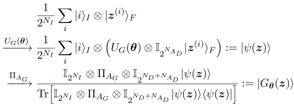
where the partial measurement $\Pi_{A_G}=(|0><0|)^{\otimes N_{A_G}}$ serves as the non-linear operation. In the sampling stage, the reconstructed image is generated similarly to the quantum patch GAN. Specifically, the $i$-th image $G_{\bm{\theta}}(\bm{z}^{(i)})$ in the batch is

$$\begin{aligned} G_{\bm{\theta}}(\bm{z}^{(i)}) ={}& \left[ P(J=0|I=i), \cdots, P(J=2^{N_D}-1|I=i) \right], \end{aligned}$$

where

$$\begin{aligned} P(J=j|I=i) ={}& \text{Tr} \left[ |i>_I |j>_F <i|_I <j|_F |G(\bm{z})><G(\bm{z})| \right] . \end{aligned}$$