Chapter 4.1 Classical Neural Networks

This content of this section corresponds to the Chapter 4.1 of our paper. Please refer to the original paper for more details.

Neural networks [@mcculloch1943logical; @gardner1998artificial; @vaswani2017attention] are computer models inspired by the structure of the human brain, designed to process and analyze complex patterns in data. Originally developed from the concept of neurons connected by weighted pathways, neural networks have become one of the most powerful tools in artificial intelligence [@lecun2015deep]. Each neuron processes its inputs by applying weights and non-linear activations, producing an output that feeds into the next layer of neurons. This structure enables neural networks to learn complex functions during training [@hornik1993some]. For example, given a dataset of images and their labels, a neural network can learn to classify categories, such as distinguishing between cats and dogs, by adjusting its parameters during training. Guided by optimization algorithms such as gradient descent [@amari1993backpropagation], the learning process allows the network to gradually reduce the error between the predicted and actual outputs, allowing it to learn the best parameters for the given task.

After nearly a century of exploration, neural networks have undergone remarkable advancements in both architectures and capabilities. The simplest model, the perceptron [@mcculloch1943logical], laid the foundation by showing how neural networks could learn to separate linearly classifiable categories. Building on this, deeper and more complex networks—such as multilayer perceptrons (MLPs) [@gardner1998artificial] and transformers [@vaswani2017attention]—have enabled breakthroughs in tasks such as autonomous driving and content generation.

Perceptron

The perceptron model, first introduced by [@mcculloch1943logical], is widely regarded as a foundational structure in artificial neural networks, inspiring architectures ranging from convolutional neural networks (CNNs) [@lecun1989handwritten] and residual neural networks (ResNets) [@he2016deep] to transformers [@vaswani2017attention]. Due to its fundamental role, we next introduce the mechanism of single-layer perceptrons.

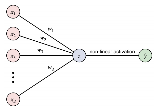
A single-layer perceptron comprises three fundamental components: input neurons, a weighted layer, and an output neuron as illustrated in Figure 1.1{reference-type=“ref” reference=“chap5_figure_perceptron”}. Given a $d$-dimensional input vector $\bm{x} \in \mathbb{R}^d$, the input layer consists of $d$ neurons, each representing the feature $\bm{x}_{i}$ for $\forall i \in [d]$. This input is processed through a weighted summation, , $$ z = \bm{w}^{\top} \bm{x},$$ where $\bm{w}^{\top}$ is the transpose of the weight vector and $z$ is the output of the weighted layer. A non-linear activation function is then applied to produce the output neuron $\hat{y}$. For the standard perceptron model, the sign function is typically used as the activation function:

$$\hat{y} = f(z) = \left\{\begin{aligned} 1, &\quad{} \text{if} \quad z \geq 0 , \\ -1, &\quad{} \text{if} \quad z < 0 . \end{aligned}\right.$$

The perceptron learns from input data by iteratively adjusting its trainable parameters $\bm{w}$. In particular, let $\mathcal{D}={(\bm{x}^{(a)}, y^{(a)})}_{a=1}^n$ be the training dataset, where $\bm{x}^{(a)}$ represents the input features of the $a$-th example, and $y^{(a)} \in {-1,1}$ denotes the corresponding label. When the perceptron outputs an incorrect prediction $\hat{y}^{(s)}$, the parameters are updated accordingly,

$$\begin{aligned} \bm{w} \leftarrow{}& \bm{w} + (y^{(s)} - \hat{y}^{(s)}) \bm{x}^{(s)}. \end{aligned}$$

The training process is repeated iteratively until the error reaches a predefined threshold.

Since the parameters are used in an inner product operation, the single-layer perceptron can be considered as a basic kernel method employing the identity feature mapping. Consequently, the single-layer perceptron can only classify linearly separable data and is inadequate for handling more complex tasks, such as the XOR problem [@rosenblatt1958perceptron]. This limitation has driven the development of advanced neural networks, such as multilayer perceptrons (MLPs) [@gardner1998artificial], which can capture non-linear relationships by incorporating non-linear activation functions and multi-layer structures.

Multilayer perceptron

The multilayer perceptron (MLP) is a fully connected neural network architecture consisting of three components: the input layer, hidden layers, and output layer, as illustrated in Figure 4.2. Similar to the single-layer perceptron, the neurons in the MLP are connected through weighted sums, followed by non-linear activation functions.

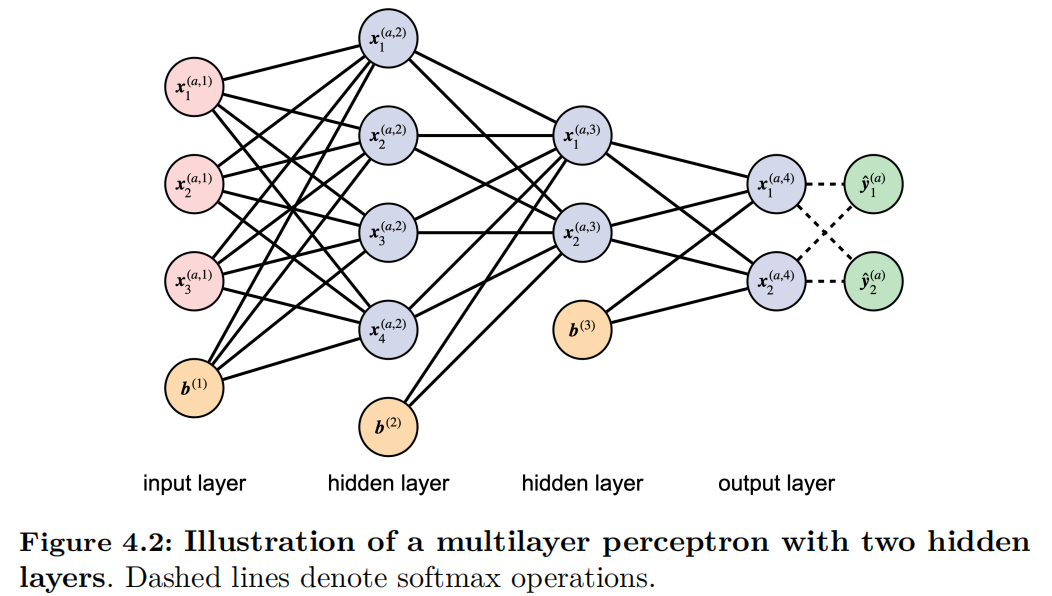
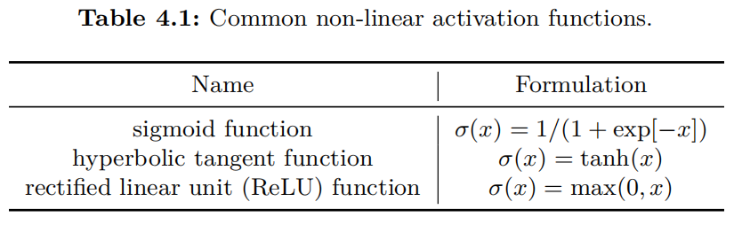
The mathematical expression of MLP is as follows. Let $\bm{x}^{(a,1)}$ be the $a$-th input data and $L$ be the number of total layers. The forward propagation is computed as follows: $$\begin{aligned} \bm{z}^{(a, \ell+1)} ={}& {W}^{(\ell)} \bm{x}^{(a, \ell)} + \bm{b}^{(\ell)} , \\ \bm{x}^{(a, \ell+1)} ={}& \sigma(\bm{z}^{(a, \ell+1)}) , \end{aligned}$$ where $\sigma$ represents the non-linear activation function and $\bm{b}^{(\ell)}$ denotes the bias term. Similar to the notation $z$ in the perceptron in Chapter 1.1.1{reference-type=“ref” reference=“chapt5:sec:classical_perceptron”}, $\bm{z}^{(a,\ell+1)}$ denotes the output of the linear sum in the $\ell+1$-th layer, which is expressed in a more generalized vector form. Therefore, the parameter for the weighted linear sum is represented in matrix form as $W^{(\ell)}$. Various methodologies have been proposed for implementing non-linear activations, with some common approaches summarized in Table 4.1.

Finally, the output given by the equation below serves as the prediction to approximate the target label $\bm{y}^{(a)}$.

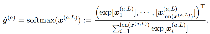
Next, we provide a toy example of binary classification to explain the MLP learning procedure. Let ${(\bm{x}^{(a)}, \bm{y}^{(a)})}_{a \in \mathcal{D}}$ be the training dataset $\mathcal{D}$, where $\bm{x}^{(a)}$ is the feature vector and $\bm{y}^{(a)} \in { (1,0)^{\top} , (0,1)^{\top} }$ is the label for two categories. Consider the MLP with one hidden layer. The prediction can be expressed as follows: $$\begin{aligned} \hat{\bm{y}}^{(a)} ={}& { softmax}(\bm{x}^{(a,3)})= { softmax} \circ \sigma \left(\bm{z}^{(a,3)} \right) \ ={}& { softmax} \circ \sigma \left({W}^{(2)} \bm{x}^{(a,2)} + \bm{b}^{(2)} \right) \ ={}& { softmax} \circ \sigma \left({W}^{(2)} \sigma \left(\bm{z}^{(a,2)} \right) + \bm{b}^{(2)} \right) \ ={}& { softmax} \circ \sigma \left({W}^{(2)} \sigma \left( W^{(1)} \bm{x}^{(a,1)} + \bm{b}^{(1)} \right) + \bm{b}^{(2)} \right) , \end{aligned}$$ where $\circ$ denotes the function composition. We use $\sigma(x)=1/(1+\exp[-x])$ as the non-linear activation function.

MLP learns from the given dataset by minimizing the loss function with respect to the parameters $\bm{\theta}=({W}^{(1)}, {W}^{(2)}, \bm{b}^{(1)}, \bm{b}^{(2)})$, which is defined as the L2 norm distance between the prediction and the label:

$$\begin{aligned} \mathcal{L}(\bm{\theta} ) ={}& \frac{1}{|\mathcal{D}|} \sum_{a \in \mathcal{D}} \mathcal{L}^{(a)}(\bm{\theta} ) = \frac{1}{2|\mathcal{D}|} \sum_{a \in \mathcal{D}} \left| \hat{\bm{y}}^{(a)}(\bm{\theta}) - \bm{y}^{(a)} \right|^2 . \end{aligned}$$

We use gradient descent with learning rate $\eta$ to optimize the parameters:

$$\bm{\theta}(t+1)=\bm{\theta}(t)-\eta \nabla_{\bm{\theta}} \mathcal{L}(\bm{\theta}(t)).$$

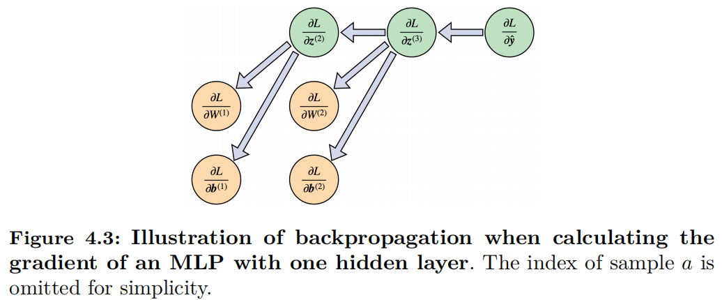
As illustrated in Figure 1.3{reference-type=“ref” reference=“chap5_figure_back_propagation”}, the gradient is computed using backpropagation [@lecun1988theoretical] shown in Figure 4.3.