Chapter 3.2 Quantum Kernel Machines

This content of this section corresponds to the Chapter 3.2 of our paper. Please refer to the original paper for more details.

Motivations for quantum kernel machines

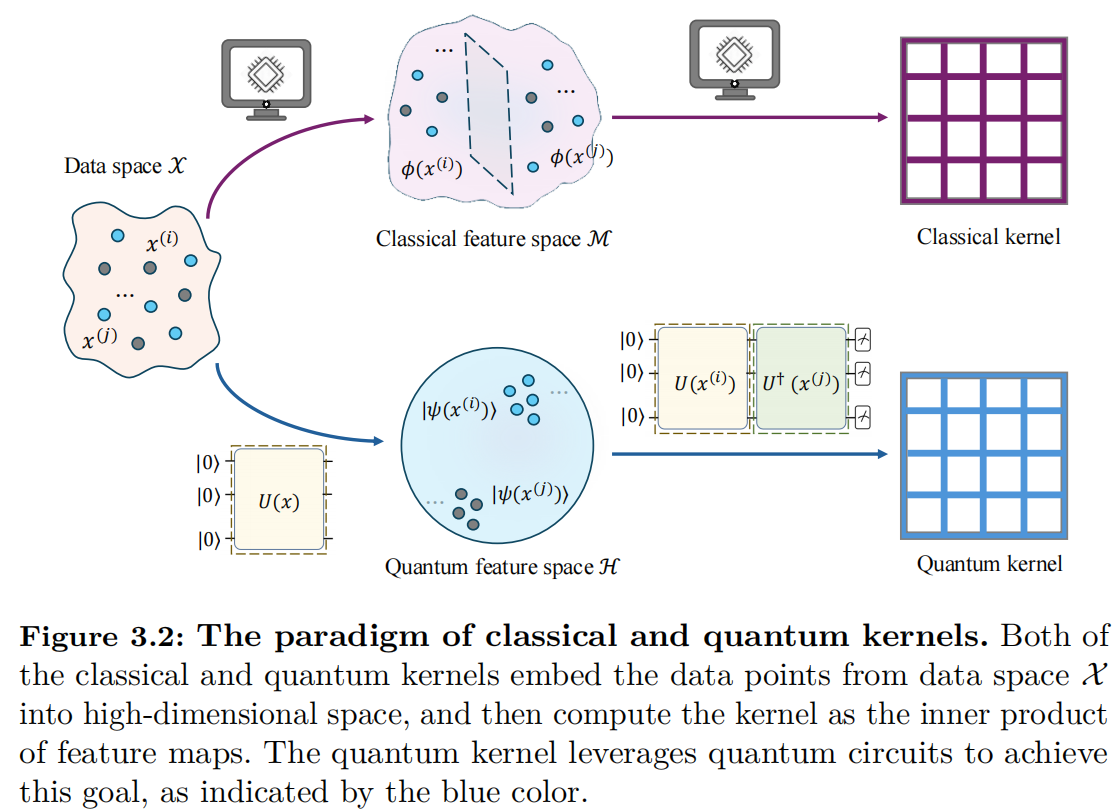
To effectively introduce quantum kernel machines, it is essential to recognize the limitations of classical kernel machines. As discussed before, classical kernel machines rely on manually tailored feature mappings, such as polynomials or radial basis functions. However, these mappings may fail to capture the complex patterns behind the dataset. Quantum kernel machines emerge as a promising alternative, as they perform feature mapping using quantum circuits, enabling them to explore exponentially larger feature spaces that are otherwise infeasible for classical computation.

Another crucial characteristic of quantum kernels is that they can be effectively implemented on noisy intermediate-scale quantum (NISQ) devices, making them a practical tool for exploring the utility of near-term quantum technologies.

Quantum feature maps and quantum kernel machines

The key difference between quantum kernel machines and classical kernel machines lies in how the feature mapping is performed. In the quantum context, a feature map refers to the injective encoding of classical data $\bm{x} \in \mathbb{R}^d$ into a quantum state $\ket{\bm{\phi}(\bm{x})}=U(\bm{x})\ket{\phi}$ on an $N$-qubit quantum register, where $U(\bm{x})$ refers to the physical operation or quantum circuit that depends on the data $\bm{x}$. This feature map is implemented on a quantum computer and produces quantum states, which are referred to as quantum feature maps.

Definition. Given an $N$-qubit quantum system initialized in state $\ket{\psi}$, let $\bm{x}\in \mathcal{X} \subset \mathbb{R}^d$ be classical data. The quantum feature map is defined as the mapping

$$ \phi:\mathcal{X} \to \mathcal{F},$$

$$\phi(\bm{x}) = \ket{\bm{\phi}(\bm{x})}\bra{\bm{\phi}(\bm{x})} = \rho(\bm{x}),$$

where $\mathcal{F}$ is the space of complex-valued $2^N \times 2^N$ matrices equipped with the Hilbert-Schmidt inner product $\braket{\rho, \sigma} = \text{Tr}(\rho \sigma)$ for $\rho, \sigma \in \mathcal{F}$. In addition, the state $\ket{\bm{\phi}(\bm{x})}$ can be implemented by applying a data-encoding quantum circuit $U(\bm{x})$ on an initial state $\ket{\psi}$.

Recall that one way of constructing kernels is adopting the inner product of the defined feature mappings. Using the Hilbert-Schmidt inner product, the quantum kernel is defined as follows.

Definition. Let $\phi$ be a quantum feature map over the domain $\mathcal{X}$. The quantum kernel is the inner product between two quantum feature maps $\rho(\bm{x}), \rho(\bm{x}’)$ for data points $\bm{x}, \bm{x}’ \in \mathcal{X}$,

$$k_Q: \mathcal{X} \times \mathcal{X} \to \mathbb{R},$$

$$k_Q(\bm{x}, \bm{x}’) = \text{Tr}(\rho(\bm{x}) \rho(\bm{x}’)) = \left|\braket{\bm{\phi}(\bm{x})|\bm{\phi}(\bm{x}’)}\right|^2.$$

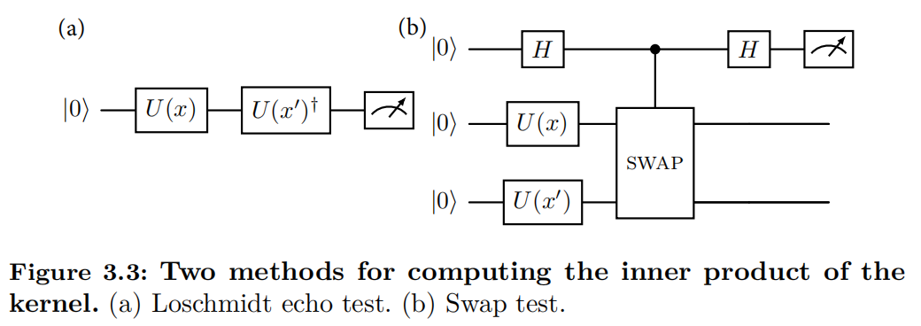
The inner product between quantum states can be efficiently estimated on quantum computers using techniques such as Loschmidt echo test [@kusumoto2021experimental] and SWAP test [@blank2020quantum]. Both methods correspond to distinct quantum circuit architectures, as illustrated in Figure 3.3.

One key merit of quantum kernels is that their derivation does not require the explicit representation of the quantum feature maps. Instead, it relies only on the construction of the associated quantum circuits. This aligns with the essence of kernel methods: while feature mappings can be computationally complex, the kernel function itself must remain efficient to evaluate.

Below, we outline the core steps for constructing a quantum kernel:

1. Quantum feature map construction: Design a data-dependent quantum circuit $U(\bm{x})$ to encode classical input data $\bm{x}$ into the amplitudes or parameters of a quantum state $\ket{\bm{\phi}(\bm{x})}=U(\bm{x})\ket{\bm{\psi}}$ where the initial state $\ket{\bm{\psi}}$ is typically $\ket{0}^{\otimes N}$.

2. Kernel evaluation: The quantum kernel is typically defined as the inner product of quantum states corresponding to two data points. Mathematically, this can be expressed as $k_Q(\bm{x},\bm{x}’)= \left| \braket{\bm{\phi}(\bm{x})|\bm{\phi}(\bm{x}’)}\right|^2$.

3. Post-processing: After executing the quantum circuit for different input pairs, measure the output and calculate the kernel matrix. This matrix will then be used in machine learning models, such as SVM.