Chapter 3.1 Classical Kernel

This content of this section corresponds to the Chapter 3.1 of our paper. Please refer to the original paper for more details.

Motivations for classical kernel machines

Before delving into kernel machines, it is essential to first understand the motivation behind kernel methods. In many machine learning tasks, particularly in classification, the goal is to find a decision boundary that best separates different classes of data. When the data is linearly separable, this boundary can be represented as a straight line (in 2D), a plane (in 3D), or a hyperplane (in higher dimensions), as illustrated in the following Figure. Mathematically, given an input space $\mathcal{X}\subset \mathbb{R}^d$ with $d\ge 1$ and a target or output space $\mathcal{Y}={+1,-1}$, we consider a training dataset $\mathcal{D}={(\bm{x}^{(i)}, {y}^{(i)})}_{i=1}^n \in (\mathcal{X} \times \mathcal{Y})^n$ where each data point $\bm{x}^{(i)} \in \mathcal{X}$ is associated with a label ${y}^{(i)} \in \mathcal{Y}$. For the dataset to be linearly separable, there must exist a vector $\bm{w} \in \mathbb{R}^{d}$ and a bias term $b\in \mathbb{R}$ such that $$\forall i\in [n], \quad {y}^{(i)}(\bm{w}^{\top} \cdot \bm{x}^{(i)}+b)\ge 0.$$ This means that a hyperplane defined by $(\bm{\omega},b)$ can perfectly separate the two classes.

Throughout the whole tutorial, we interchangeably use the following notations to denote the inner product of two vectors $\bm{a}$ and $\bm{b}$, i.e., [complete. $\langle \cdot, \cdot \rangle$, $\braket{\cdot|\cdot}$, $\bm{a}\cdot \bm{b}$, $\bm{a}^{\dagger} \bm{b}$]

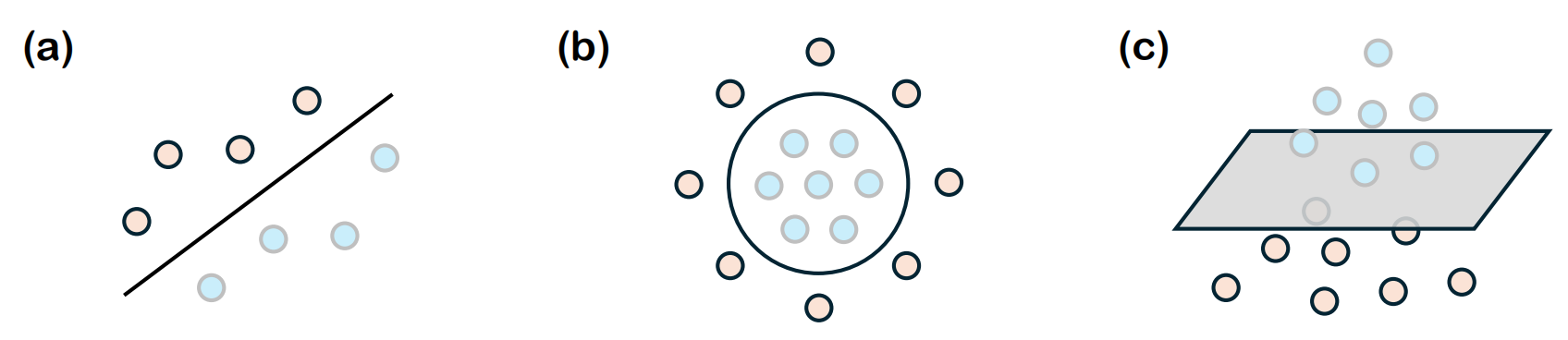
However, in real-world scenarios, data is often not linearly separable, as shown in the Figure(b). The decision boundary required to separate classes may be curved or highly complex. Traditional linear models struggle with such non-linear data because they are inherently limited to creating only linear decision boundaries. This limitation highlights the need for more flexible approaches.

To address the challenge of non-linear data, one effective strategy is to transform the input data into a higher-dimensional space where the data may become linearly separable. This transformation is known as feature mapping, denoted by $$ \bm{\phi}:\bm{x} \to \phi(\bm{x})\in \mathbb{R}^D,$$ where the original input space $\mathcal{X}$ is mapped to a higher-dimensional feature space $\mathbb{R}^D$ with $D\ge d$. The idea is that, in this higher-dimensional space, complex patterns in the original data can be more easily identified using linear models.

However, explicitly computing the feature map $\bm{\phi}(\bm{x})$ can be computationally expensive, especially if the feature space is high-dimensional or even infinite-dimensional. Fortunately, many machine learning algorithms for tasks like classification or regression depend primarily on the inner product between data points. In the feature space, this inner product is given by $\braket{\bm{\phi}(\bm{x}^{(i)}),\bm{\phi}(\bm{x}^{(j)})}$.

To circumvent the computational cost of explicitly calculating the feature map, we can use a kernel function. A kernel function $k(\bm{x}^{(i)}, \bm{x}^{(j)})$ is defined as $$ k(\bm{x}^{(i)}, \bm{x}^{(j)})=\braket{\bm{\phi}(\bm{x}^{(i)}),\bm{\phi}(\bm{x}^{(j)})}.$$ This allows us to compute the inner product in the higher-dimensional feature space indirectly, without ever having to compute $\bm{\phi}(\bm{x})$ explicitly. This approach is commonly known as the kernel trick.

By using the kernel function directly within algorithms, we avoid the computational overhead of working in a high-dimensional space. The collection of kernel values for a dataset forms the kernel matrix (or Gram matrix), where each entry is given by $k(\bm{x}^{(i)}, \bm{x}^{(j)})$. This matrix is central to many kernel-based algorithms, as it captures the pairwise similarities between all training data points.

Throughout this tutorial, we use the notations $\mathcal{O}$ and $\Omega$ to represent the asymptotic upper and lower bounds, respectively, on the growth rate of a term, ignoring constant factors and lower-order terms.

Kernel construction

To utilize the kernel trick in machine learning algorithms, it is essential to construct valid kernel functions. One approach is to start with a feature mapping $\bm{\phi}(\bm{x})$ and then derive the corresponding kernel. For a one-dimensional input space, the kernel function is defined as $$k(x, x’) = \langle \bm{\phi}(\bm{x})^{\top}, \bm{\phi}(\bm{x}’) \rangle = \sum_{i=1}^D \langle \bm{\phi}_i(\bm{x}), \bm{\phi}_i(\bm{x}’) \rangle,$$ where $\bm{\phi}_i(\bm{x})$ are the basis functions of the feature map.

Alternatively, kernels can be constructed directly without explicitly defining a feature map. In this case, we must ensure that the chosen function is a valid kernel, meaning it corresponds to an inner product in some (possibly infinite-dimensional) feature space. The validity of a kernel function is guaranteed by Mercer’s condition.