Chapter 1 Introduction of QML

Introduction

The advancement of computational power has always been a driving force behind every major industrial revolution. The invention of the modern computer, followed by the central processing unit (CPU), led to the “digital revolution”, transforming industries through process automation and the rise of information technology. More recently, the development of graphical processing units (GPUs) has powered the era of artificial intelligence (AI) and big data, enabling breakthroughs in areas such as intelligent transportation systems, autonomous driving, scientific simulations, and complex data analysis. However, as we approach the physical and practical limits of Moore’s law—the principle that the number of transistors on a chip doubles approximately every two years—traditional computing devices like CPUs and GPUs are nearing the end of their scaling potential. The ever-growing demand for computational power, driven by the exponential increase in data and the complexity of modern applications, necessitates new computing paradigms. Among the leading candidates to meet these challenges are quantum computers [@feynman2017quantum], which leverage the unique principles of quantum mechanics such as superposition and entanglement to process information in ways that classical systems cannot, with the potential to revolutionize diverse aspects of daily life.

One of the most concrete and direct ways to understand the potential of quantum computers is through the framework of complexity theory [@watrous2008quantum]. Theoretical computer scientists have demonstrated that quantum computers can efficiently solve problems within the $\mathop{\mathrm{\mathsf{BQP}}}$ (Bounded-Error Quantum Polynomial Time) complexity class, meaning these problems can be solved in polynomial time by a quantum computer. In contrast, classical computers are limited to efficiently solving problems within the $\mathop{\mathrm{\mathsf{P}}}$ (Polynomial Time) complexity class. While it is widely believed, though not proven, that $\mathop{\mathrm{\mathsf{P}}}\subseteq \mathop{\mathrm{\mathsf{BQP}}}$, this suggests that quantum computers can provide exponential speedups for certain problems in $\mathop{\mathrm{\mathsf{BQP}}}$ that are intractable for classical machines.

A prominent example of such a problem is large-number factorization, which forms the basis of RSA cryptography. Shor’s algorithm [@shor1999polynomial], a quantum algorithm, can factor large numbers in polynomial time, while the most efficient known classical factoring algorithm requires super-polynomial time. For instance, breaking an RSA-2048 bit encryption key would take a classical computer approximately 300 trillion years, whereas an ideal quantum computer could complete the task in around 10 seconds. However, constructing ‘ideal’ quantum computers remains a significant challenge. As will be discussed in later chapters, based on current fabrication techniques, this task could potentially be completed in approximately 8 hours using a noisy quantum computer with a sufficient number of qubits—the fundamental units of quantum computation [@gidney2021factor].

The convergence of the computational power offered by quantum machines and the limitations faced by AI models has led to the rapid emergence of the field: quantum machine learning (QML) [@biamonte2017quantum]. In particular, the challenges in modern AI stem from the neural scaling law [@kaplan2020scaling], which posits that “bigger is often better.” Since 2020, this principle has driven the development of increasingly colossal models, featuring more complex architectures and an ever-growing number of parameters. However, this progress comes at an immense cost. For instance, training a model like ChatGPT on a single GPU would take approximately 355 years, while the cloud computing costs for training such large models can reach tens of thousands of dollars.

These staggering costs present a critical barrier to the future growth of AI. Quantum computing, celebrated for its extraordinary computational capabilities, holds the potential to overcome these limitations. It offers the possibility of advancing models like generative pre-trained transformers (GPTs) and accelerating progress toward artificial general intelligence (AGI). Quantum computing, and more specifically QML, represents a paradigm shift, moving from the classical “it from bit” framework to the quantum “it from qubit” era, with the potential to reshape the landscape of AI and computational science.

A First Glimpse of Quantum Machine Learning

So, what exactly is quantum machine learning (QML)? In its simplest terms, the focus of this tutorial on QML can be summarized as follows (see Chapter 1.1.3{reference-type=“ref” reference=“chapter1:explored-task-QML”} for the systematic overview).

QML explores learning algorithms that can be executed on quantum computers to accomplish specified tasks with potential advantages over classical implementations.

The three key elements in the above interpretation are: quantum processors, specified tasks, and advantages. In what follows, let us elucidate the specific meaning of each of these terms, providing the necessary foundation for a deeper understanding of the mechanisms and potential of QML.

Quantum computers

The origins of quantum computing can be traced back to 1980 when Paul Benioff introduced the quantum Turing machine [@benioff1982quantum], a quantum analog of the classical Turing machine designed to describe computational models through the lens of quantum theory. Since then, several models of quantum computation have emerged, including circuit-based quantum computation [@nielsen2010quantum], one-way quantum computation [@raussendorf2001one], adiabatic quantum computation [@albash2018adiabatic], and topological quantum computation [@kitaev2003fault]. All of them have been shown to be computationally equivalent to the quantum Turing machine, meaning that a perfect implementation of any one of these models can simulate the others with no more than polynomial overhead. Given the prominence of circuit-based quantum computers in both the research and industrial communities and their rapid advancement, this tutorial will focus primarily on this model of quantum computing.

Quantum computing gained further momentum in the early 1980s when physicists faced an exponential increase in computational overhead while simulating quantum dynamics, particularly as the number of particles in a system grew. This “curse of dimensionality” prompted Yuri Manin and Richard Feynman to independently propose leveraging quantum phenomena to build quantum computers, arguing that such devices would be far more efficient for simulating quantum systems than classical computers.

However, as a universal computing device, the potential of quantum computers extends well beyond quantum simulations. In the 1990s, @shor1999polynomial developed a groundbreaking quantum algorithm for large-number factorization, posing a serious threat to widely used encryption protocols such as RSA and Diffie–Hellman. In 1996, Grover’s algorithm demonstrated a quadratic speedup for unstructured search problems [@grover1996fast], a task with broad applications. Since then, the influence of quantum computing has expanded into a wide range of fields, with new quantum algorithms being developed to achieve runtime speedups in areas such as finance [@herman2023quantum], drug design [@santagati2024drug], optimization [@abbas2024challenges], and, most relevant to this tutorial, machine learning.

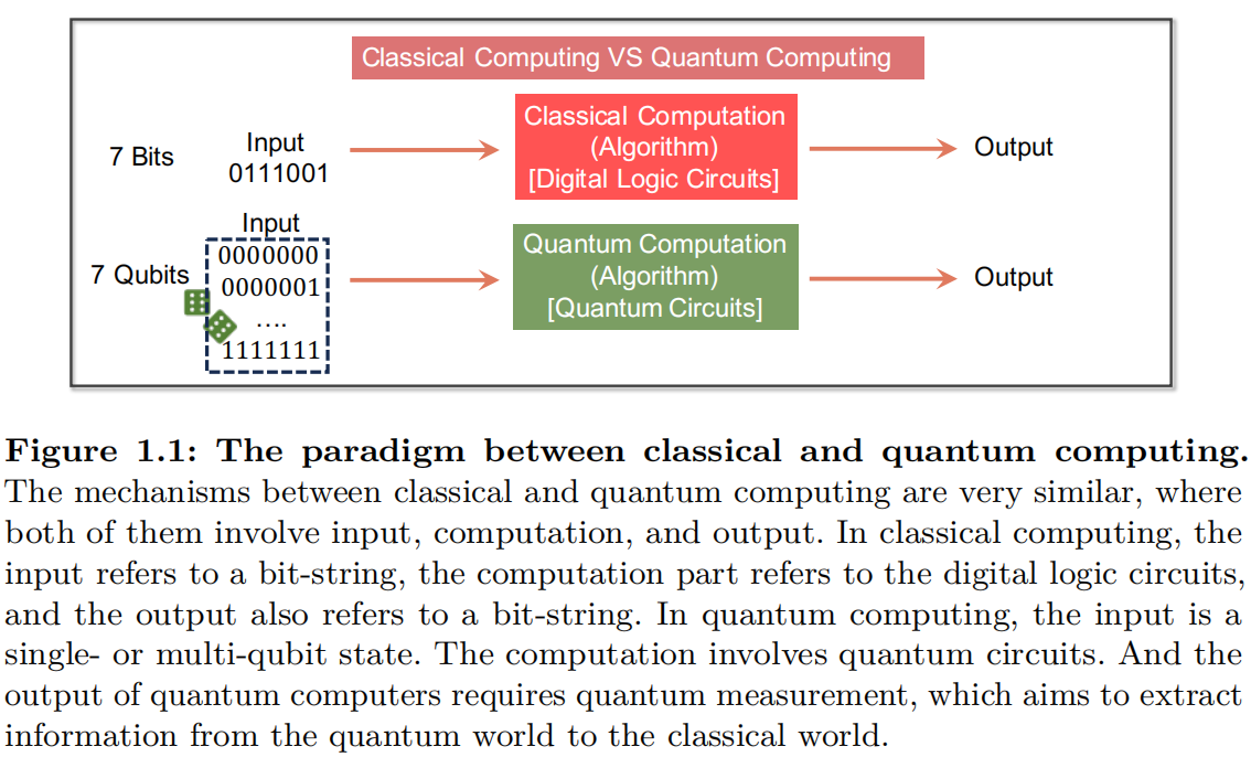
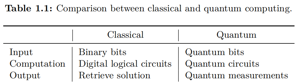
An intuitive way to understand why quantum computers can outperform classical computers is by comparing their fundamental components. As illustrated in Figure 1.1, both types of computers consist of three fundamental components: input, the computational process, and the output. The implementation of these three components in classical and quantum computing is summarized in Table 1.1.

The advantages of quantum computers stem primarily from the key distinctions between classical bits and quantum bits (qubits), as well as between digital logic circuits and quantum circuits, as outlined below:

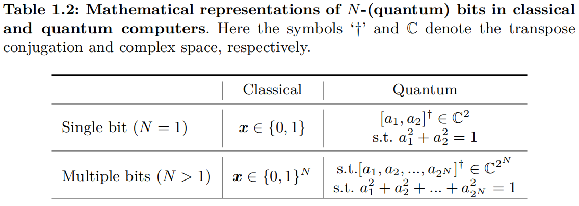
Bits versus Qubits. A classical bit is a binary unit that takes on a value of either $0$ or $1$. In contrast, a quantum bit, or qubit, can exist in a superposition of both $0$ and $1$ simultaneously, represented by a two-dimensional vector where the entries correspond to the probabilities of the qubit being in each state.

Furthermore, while classical bits follow the Cartesian product rule, qubits adhere to the tensor product rule. This distinction implies that an $N$-qubit system is described by a $2^N$-dimensional vector, allowing quantum systems to encode information exponentially with $N$—far surpassing the capacity of classical bits. Table 1.4{reference-type=“ref” reference=“tab:chapt1-math-single-multi-qubits”} summarizes the mathematical expressions of classical and quantum bits.

Digital logic circuits versus quantum circuits. Classical computers rely on digital logic circuits composed of logic gates that perform operations on bits in a deterministic manner, as illustrated in Figure 1.1. In contrast, quantum circuits consist of quantum gates, which act on single or multiple qubits to modify their states—the probability amplitudes $a_1,…, a_{2^N}$, as shown in Table 1.2. Owing to the universality of quantum gates, for any given input qubit state, there always exists a specific quantum circuit capable of transforming the input state into one corresponding to the target solution—a particular probability distribution. For certain probability distributions, a quantum computer can use a polynomial number of quantum gates relative to the qubit count $N$ to generate the distribution, whereas classical computers require an exponential number of gates with $N$ to achieve the same result. This difference underpins the quantum advantage.
The readout process in quantum computing differs fundamentally from that in classical computing, as it involves quantum measurements, which extract information from a quantum system and translate it into a form that can be interpreted by classical systems. For problems in quantum physics and chemistry, quantum measurements can reveal far more useful information than classical simulations of the same systems, enabling significant runtime speedups in obtaining the desired physical properties.

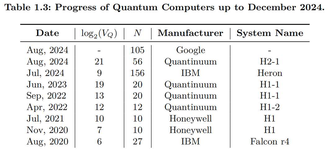
The formal definitions of quantum computing are presented in Chapter 2. As we will see, the power of quantum computers is primarily determined by two factors: the number of qubits and the quantum gates, as well as their respective qualities. The term “qualities” refers to the fact that fabricating quantum computers is highly challenging, as both qubits and quantum gates are prone to errors. These qualities are measured using various physical metrics. One commonly used metric is quantum volume $V_Q$ [@cross2019validating], which quantifies a quantum computer’s capabilities by accounting for both its error rates and overall performance. Mathematically, the quantum volume represents the maximum size of square quantum circuits that the computer can successfully implement to achieve the heavy output generation problem, i.e., $$\log_2(V_Q) = \arg\max_{m} \min(m, d(m)),$$ where $m\leq N$ is a number of qubits selected from the given $N$-qubit quantum computer, and $d(m)$ is the number of qubits in the largest square circuits for which we can reliably sample heavy outputs with probability greater than $2/3$. The heavy output generation problem discussed here stems from proposals aimed at demonstrating quantum advantage. That is, if a quantum computer is of sufficiently high quality, we should expect to observe heavy outputs frequently across a range of random quantum circuit families. For illustration, Table 1.3 summarizes the progress of quantum computers as of 2024.

Note that quantum volume is not the unique metric for evaluating the performance of quantum computers. There are several other metrics that assess the power of quantum processors from different perspectives. For instance, Circuit Layer Operations Per Second (CLOPS) [@wack2021quality] measures the computing speed of quantum computers, reflecting the feasibility of running practical calculations that involve a large number of quantum circuits. Additionally, effective quantum volume [@kechedzhi2024effective] provides a more nuanced comparison between noisy quantum processors and classical computers, considering factors such as error rates and noise levels. These metrics, among others, offer a more comprehensive understanding of the strengths and limitations of quantum computers across various applications. :::

Different measures of quantum advantages

What do we mean when we refer to quantum advantage? Broadly, quantum advantage is demonstrated when quantum computers can solve a problem more efficiently than classical computers. However, the notion of “efficiency” in this context is not uniquely defined.

The most common measure of efficiency is runtime complexity. By harnessing quantum effects, certain computations can be accelerated significantly—sometimes even exponentially—enabling tasks that are otherwise infeasible for classical computers. A prominent example is Shor’s algorithm, which achieves an exponential speedup in large-number factorization relative to the best classical algorithms. In terms of runtime complexity, the quantum advantage is achieved when the upper bound of a quantum algorithm’s runtime for a given task is lower than the theoretical lower bound of all possible classical algorithms for the same task.

In quantum learning theory [@arunachalam2017guest], efficiency can also be measured by sample complexity, particularly within the Probably Approximately Correct ($\mathop{\mathrm{\mathsf{PAC}}}$) learning framework, which is central to this tutorial. In this context, sample complexity is defined as the number of interactions (e.g., quires of target quantum systems or measurements) required for a learner to achieve a desired prediction accuracy below a specified threshold. Here, the quantum advantage is realized when the upper bound on the sample complexity of a quantum learning algorithm for a given task is lower than the lower bound of all classical learning algorithms. While low sample complexity is a necessary condition for efficient learning, it does not guarantee practical efficiency alone; for example, identifying useful training examples within a small sample size may still require substantial computational time.

Difference of sample complexity in classical and quantum ML. In classical ML, sample complexity typically refers to the number of training examples required for a model to generalize effectively, such as the number of labeled images needed to train an image classifier. In quantum ML, however, sample complexity can take on varied meanings depending on the context, as shown below.

Quantum state tomography (see Chapter 2.3). Here the sample complexity refers to the number of measurements required to accurately reconstruct the quantum state of a system.
Evaluation of the generalization ability of quantum neural networks (see Chapter 4.4). Here the sample complexity refers to the number of input-output pairs needed to train the network to approximate a target function, similar to classical ML.
Quantum system learning. Here the sample complexity often refers to the number of queries to interact with the target quantum system, such as the number of times a system must be probed to learn its Hamiltonian dynamics.

In addition to sample complexity, another commonly used measure in quantum learning theory is quantum query complexity, particularly within the frameworks of quantum statistical learning and quantum exact learning. As these frameworks are not the primary focus of this tutorial, interested readers are referred to [@anshu2024survey] for a more detailed discussion.

Quantum advantage can be pursued through two main approaches. The first involves identifying problems with quantum circuits that demonstrate provable advantages over classical counterparts in the aforementioned measures [@harrow2017quantum]. Such findings deepen our understanding of quantum computing’s potential and expand its range of applications. However, these quantum circuits often require substantial quantum resources, which are currently beyond the reach of near-term quantum computers. Additionally, for many tasks, analytically determining the upper bound of classical algorithm complexities is challenging.

These challenges have motivated a second approach: demonstrating that current quantum devices can perform accurate computations on a scale that exceeds brute-force classical simulations—a milestone known as “quantum utility.” Quantum utility refers to quantum computations that yield reliable, accurate solutions to problems beyond the reach of brute-force classical methods and otherwise accessible only through classical approximation techniques [@kim2023evidence]. This approach represents a step toward practical computational advantage with noise-limited quantum circuits. Reaching the era of quantum utility signifies that quantum computers have attained a level of scale and reliability enabling researchers to use them as effective tools for scientific exploration, potentially leading to groundbreaking new insights.

Explored tasks in quantum machine learning

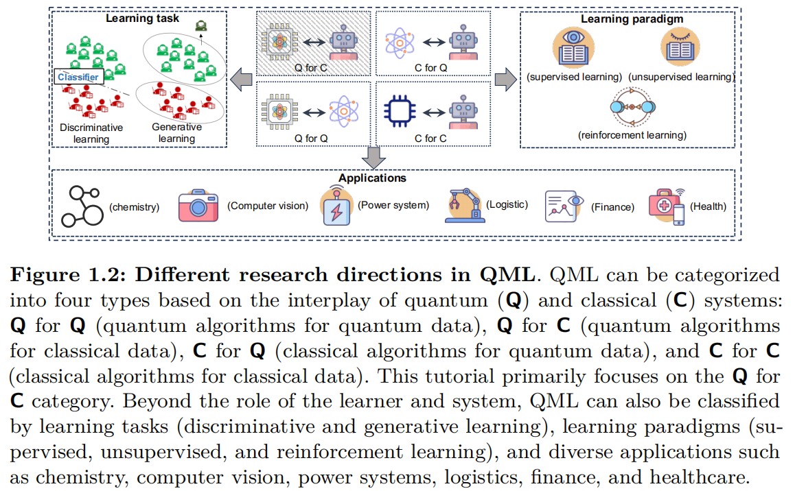
What are the main areas of focus in QML? QML research is extensive and can be broadly divided into four primary sectors, each defined by the nature of the computing resources (whether the computing device is quantum ([Q]) or classical ([C])) and the type of data involved (whether generated by a quantum ([Q]) or classical ([C]) system). The explanations of these four sectors are as follows.

[CC] Sector. The [CC] sector refers to classical data processed on classical systems, representing traditional machine learning. Here, classical ML algorithms run on classical processors (e.g., CPUs and GPUs) and are applied to classical datasets. A typical example is using neural networks to classify images of cats and dogs.
[CQ] Sector: The [CQ] sector involves using classical ML algorithms on classical processors to analyze quantum data collected from quantum systems. Typical examples include applying classical neural networks to classify quantum states, estimating properties of quantum systems from measurement data, and employing classical regression models to predict outcomes of quantum experiments.
[QC] Sector. The [QC] sector involves developing QML algorithms that run on quantum processors (QPUs) to process classical data. In this context, quantum computing resources are leveraged to enhance or accelerate the analysis of classical datasets. Typical examples include applying QML algorithms, such as quantum neural networks and quantum kernels, to improve pattern recognition in image analysis.
[QQ] Sector. The [QQ] sector involves developing QML algorithms executed on QPUs to process quantum data. In this context, quantum computing resources are leveraged to reduce the computational cost of analyzing and understanding complex quantum systems. Typical examples include using quantum neural networks for quantum state classification and applying quantum-enhanced algorithms to simulate quantum many-body systems.

The classification above is not exhaustive. As illustrated in Figure 1.2, each sector can be further subdivided based on various learning paradigms, such as discriminative vs. generative learning or supervised, unsupervised, and semi-supervised learning. Additionally, each sector can be further categorized according to different application domains, such as finance, healthcare, and logistics.

The primary focus of this tutorial is on the [QC] and [QQ] sectors. For more details on [CQ], interested readers can refer to [@schuld2015introduction; @dunjko2018machine; @carleo2019machine].

Progress of Quantum Machine Learning

Huge efforts have been made to the [QC] and [QQ] sectors to determine which tasks and conditions allow QML to offer computational advantages over classical machine learning. In this regard, to provide a clearer understanding of QML’s progress, it is essential to first review recent advancements in quantum computers, the foundational substrate for quantum algorithms.

Progress of quantum computers

The novelty and inherent challenges of utilizing quantum physics for computation have driven the development of various computational architectures, giving rise to the formalized concept of circuit-based quantum computers. In pursuit of this goal, numerous companies and organizations are striving to establish their architecture as the leading approach and to be the first to demonstrate practical utility or quantum advantage on a large-scale quantum device.

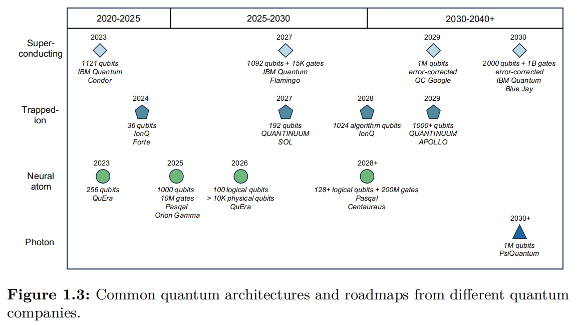
Common architectures currently include superconducting qubits (employed by IBM and Google), ion-trap systems (pioneered by IonQ), and Rydberg atom systems (developed by QuEra), each offering distinct advantages [@cheng2023noisy]. Specifically, superconducting qubits excel in scalability and fast gate operations [@huang2020superconducting], while ion-trap systems are known for their high coherence times, precise control over individual qubits, and full connectivity of all qubits [@bruzewicz2019trapped]. Moreover, Rydberg atom systems enable flexible qubit connectivity through highly controllable interactions [@morgado2021quantum]. Besides these architectures, integrated photonic quantum computers are emerging as promising alternatives for robust and scalable quantum computation.

Despite recent advances, today’s quantum computers remain highly sensitive to environmental noise and prone to quantum decoherence, lacking the stability needed for fault-tolerant operation. This results in qubits, quantum gates, and quantum measurements that are inherently imperfect, introducing errors that can lead to incorrect outputs. To capture this stage in quantum computing, John Preskill coined the term “noisy intermediate-scale quantum” ([NISQ]) era [@preskill2018quantum], which describes the current generation of quantum processors. These processors feature up to thousands of qubits, but their capabilities are restricted with error-prone gates and limited coherence times.

In the [NISQ] era, notable achievements have been made alongside new challenges. Industrial and academic teams, such as those at Google and USTC, have demonstrated quantum advantages on specific sampling tasks, where the noisy quantum computers they fabricated outperform classical computers in computational efficiency [@arute2019quantum; @wu2021strong]. However, most quantum algorithms that theoretically offer substantial runtime speedups depend on fault-tolerant, error-free quantum systems—capabilities that remain beyond the reach of current technology.

At this pivotal stage, the path forward in quantum computing calls for progress on both hardware and algorithmic fronts.

On the hardware side, it is essential to continuously improve qubit count, coherence times, gate fidelities, and the accuracy of quantum measurements across various quantum architectures. Once the number and quality of qubits surpass certain thresholds, quantum error correction codes can be implemented [@nielsen2010quantum], paving the way for fault-tolerant quantum computing ([FTQC]). Broadly, quantum error correction uses redundancy and entanglement to detect and correct errors without directly measuring the quantum state, thus preserving coherence. Advancements in quantum processors will enable a progression from the [NISQ] era to the early [FTQC] era, ultimately reaching the fully [FTQC] era.

On the algorithmic side, two key questions must be addressed:

How can [NISQ] devices be utilized to perform meaningful computations with practical utility?
What types of quantum algorithms can be executed on early fault-tolerant and fully fault-tolerant quantum computers to realize the potential of quantum computing in real-world applications?

Progress on either question could have broad implications. A positive answer to (Q1) would suggest that [NISQ] quantum computers have immediate practical applicability, while advancements in (Q2) would expand the scope and impact of quantum computing as more robust, fault-tolerant systems become feasible. In the following two sections, we examine recent progress in QML concerning these two questions.

Progress of quantum machine learning under FTQC

A key milestone in [FTQC]-based QML algorithms is the quantum linear equations solver introduced by @harrow2009quantum. Many machine learning models rely on solving linear equations, a computationally intensive task that often dominates the overall runtime due to the polynomial scaling of complexity with matrix size. The HHL algorithm provides a breakthrough by reducing runtime complexity to poly-logarithmic scaling with matrix size, given that the matrix is well-conditioned and sparse. This advancement is highly significant for AI, where datasets frequently reach sizes in the millions or even billions.

The exponential runtime speedup achieved by the HHL algorithm has garnered significant attention from the research community, highlighting the potential of quantum computing in AI. Following this milestone, a body of work has emerged that employs the quantum matrix inversion techniques developed in HHL (or its variants) as subroutines in the design of various [FTQC]-based QML algorithms, offering runtime speedups over their classical counterparts [@montanaro2016quantum; @dalzell2023quantum]. Notable examples include quantum principal component analysis [@lloyd2014quantum] and quantum support vector machines [@rebentrost2014quantum].

Another milestone in [FTQC]-based QML algorithms is the quantum singular value transformation (QSVT), proposed by @gilyenquantum2019. QSVT enables polynomial transformations of the singular values of a linear operator embedded within a unitary matrix, offering a unifying framework for various quantum algorithms. It has connected and enhanced a broad range of quantum techniques, including amplitude amplification, quantum linear system solvers, and quantum simulation methods. Compared to the HHL algorithm for solving linear equations, QSVT provides improved scaling factors, making it a more efficient tool for addressing these problems in the context of QML.

In addition to advancements in linear equation solving, another promising line of research in [FTQC]-based QML focuses on leveraging quantum computing to enhance deep neural networks (DNNs) rather than traditional machine learning models. This research track has two main areas of focus. The first is the acceleration of DNN optimization, with notable examples including the development of efficient quantum algorithms for dissipative differential equations to expedite (stochastic) gradient descent, as well as Quantum Langevin dynamics for optimization [@chen2023quantum; @liu2024towards]. The second area centers on advancing Transformers using quantum computing. In Chapter 5, we will discuss in detail how quantum computing can be employed to accelerate Transformers during the inference stage.

However, there are several critical caveats of the HHL-based QML algorithms. First, the assumption of efficiently preparing the quantum states corresponding to classical data runtime is very strong and may be impractical in the dense setting. Second, the obtained result $\bm{x}$ is still in the quantum form $\ket{\bm{x}}$. Note that extracting one entry of $\ket{\bm{x}}$ into the classical form requires $O(\sqrt{N})$ runtime, which collapses the claimed exponential speedups. The above two issues amount to the read-in and read-out bottlenecks in QML [@aaronson2015read]. The last caveat is that the employed strong quantum input model such as quantum random access memory (QRAM) [@giovannetti2008quantum] leads to an inconclusive comparison. Through exploiting a classical analog of QRAM as the input model, there exist efficient classical algorithms to solve recommendation systems in poly-logarithmic time in the size of input data.

Progress of quantum machine learning under NISQ

The work conducted by @havlivcek2019supervised marked a pivotal moment for QML in the [NISQ] era. This study demonstrated the implementation of quantum kernel methods and quantum neural networks (QNNs) on a 5-qubit superconducting quantum computer, highlighting potential quantum advantages from the perspective of complexity theory. Unlike the aforementioned [FTQC] algorithms, quantum kernel methods and QNNs are flexible and can be effectively adapted to the limited quantum resources available in the [NISQ] era. These demonstrations, along with advancements in quantum hardware, sparked significant interest in exploring QML applications using [NISQ] quantum devices. We will delve into quantum kernel methods and QNNs in Chapter 3 and Chapter 4, respectively.

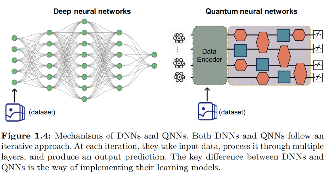
A quantum neural network (QNN) is a hybrid model that leverages quantum computers to implement trainable models similar to classical neural networks, while using classical optimizers to complete the training process.

As shown in Figure 1.4, the mechanisms of QNNs and deep neural networks (DNNs) are almost the same, whereas the only difference is the way of implementing the trainable model. This difference gives the potential of quantum learning models to solve complex problems beyond the reach of classical neural networks, opening new frontiers in many fields. Roughly speaking, research in QNNs and quantum kernel methods has primarily focused on three key areas: (I) quantum learning models and applications, (II) the adaptation of advanced AI topics to QML, and (III) theoretical foundations of quantum learning models. A brief overview of each category is provided below.

(I) [Quantum learning models and applications]. This category focuses on implementing various DNNs on [NISQ] quantum computers to tackle a wide range of tasks.

From a model architecture perspective, quantum analogs of popular classical machine learning models have been developed, including quantum versions of multilayer perceptrons (MLPs), autoencoders, convolutional neural networks (CNNs), recurrent neural networks (RNNs), extreme learning machines, generative adversarial networks (GANs), diffusion models, and Transformers. Some of these QNN structures have even been validated on real quantum platforms, demonstrating the feasibility of applying quantum algorithms to tasks traditionally dominated by classical deep learning [@cerezo2021variational; @li2022recent; @tian2023recent].

From an application perspective, QML models implemented on [NISQ] devices have been explored across diverse fields, including fundamental science, image classification, image generation, financial time series prediction, combinatorial optimization, healthcare, logistics, and recommendation systems. These applications demonstrate the broad potential of QML in the [NISQ] era, though achieving full quantum advantage in these areas remains an ongoing challenge [@bharti2022noisy; @cerezo2022challenges].

(II) [Adaptation of advanced AI topics to QML]. Beyond model design, advanced topics from AI have been extended to QML, aiming to enhance the performance and robustness of different QML models. Examples include quantum architecture search [@du2022quantum] (the quantum equivalent of neural architecture search), advanced optimization techniques [@stokes2020quantum], and pruning methods to reduce the complexity of quantum models [@sim2021adaptive; @wang2023symmetric]. Other areas of active research include adversarial learning [@Lu2020Quantum], continual learning [@Jiang_2022Quantum], differential privacy [@du2021quantum; @Watkins2023Quantum], distributed learning [@du2022distributed], federated learning [@ren2023towards], and interpretability within the context of QML [@pira2024interpretability]. These techniques have the potential to significantly improve the efficiency and effectiveness of QML models, addressing some of the current limitations of [NISQ] devices.

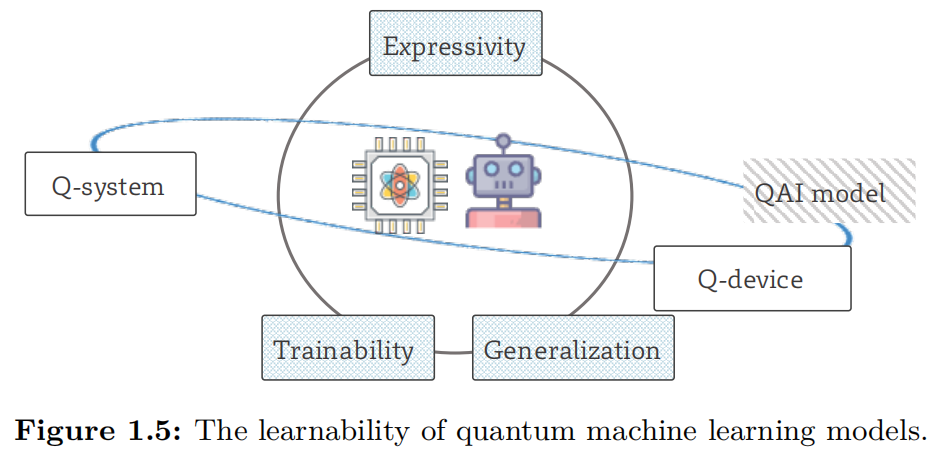
(III) [Theoretical foundations]. Quantum learning theory [@banchi2023statistical] has garnered increasing attention, aiming to compare the capabilities of different QML models and to identify the theoretical advantages of QML over classical machine learning models. As shown in Figure 1.4{reference-type=“ref” reference=“fig:chapter1-QLT-overview”}, the learnability of QML models can be evaluated across three key dimensions: expressivity, trainability, and generalization capabilities. Below, we provide a brief overview of each measure.

Trainability. This area examines how the design of QNNs influences their convergence properties, including the impact of system noise and measurement errors on the ability to converge to local or global minima.
Expressivity. Researchers investigate how the number of parameters and the structure of QNNs affect the size of the hypothesis space they can represent. A central question is whether QNNs and quantum kernels can efficiently represent functions or patterns that classical neural networks cannot, thereby offering potential quantum advantage.
Generalization. This focuses on understanding how the gap between training and test error evolves with the size of the dataset, the structure of QNNs or quantum kernels, and the number of parameters. The goal is to determine whether QML models can generalize more effectively than classical models, particularly in the presence of noisy data or when training data is limited.

The combination of advancements in model design, application domains, and theoretical understanding is driving the progress of QML in the NISQ era. Although the field is still in its early stages, the progress achieved thus far provides promising insights into the potential of quantum computing to enhance conventional AI. As quantum hardware continues to evolve, further breakthroughs are expected, potentially unlocking new possibilities for practical QML applications.

It is important to note that QNNs and quantum kernel methods can also be considered [FTQC] algorithms when executed on fully fault-tolerant quantum computers. The reason these algorithms are discussed in the context of [NISQ] devices is their flexibility and robustness, making them well-suited to the limitations of current quantum hardware.

A brief review of quantum machine learning

Unlike quantum hardware, where the number of qubits has rapidly scaled from zero to thousands, the development of QML algorithms—and quantum algorithms more broadly—has taken an inverse trajectory, transitioning from [FTQC] to [NISQ] devices. This shift reflects the move from idealized theoretical frameworks to practical implementations. The convergence of quantum hardware and QML algorithms, where the quantum resources required by these algorithms become attainable on real quantum computers, enables researchers to experimentally evaluate the power and limitations of various quantum algorithms.

Based on the minimum quantum resources required to complete learning tasks, we distinguish between [FTQC] algorithms, and [NISQ] algorithms, including QNNs and quantum kernel methods. [FTQC]-based QML algorithms necessitate error-corrected quantum computers with tens of billions of qubits—an achievement that remains far from realization. In contrast, QNNs and quantum kernels are more flexible and can be executed on both [NISQ] and [FTQC] devices, depending on the available resources.

As quantum hardware continues to progress, the development of QML algorithms must evolve in tandem. A promising direction is to integrate [FTQC] algorithms with QNNs and quantum kernel methods, creating new QML algorithms that can be run on current quantum processors while offering enhanced quantum advantages across various tasks.